Is It Different to Read a Chi Square Table Than a T Test Table
Chi-square examination of independence in R
- Introduction
- Data
- Chi-square test of independence in R
- Conclusion and interpretation
- Combination of plot and statistical test

Introduction
This article explains how to perform the Chi-square test of independence in R and how to interpret its results. To learn more almost how the exam works and how to do information technology by hand, I invite you to read the article "Chi-square test of independence past hand".
To briefly epitomize what have been said in that article, the Chi-square exam of independence tests whether there is a relationship between two categorical variables. The nada and alternative hypotheses are:
- \(H_0\) : the variables are contained, there is no relationship between the two categorical variables. Knowing the value of one variable does non aid to predict the value of the other variable
- \(H_1\) : the variables are dependent, there is a relationship between the two chiselled variables. Knowing the value of one variable helps to predict the value of the other variable
The Chi-foursquare test of independence works by comparing the observed frequencies (so the frequencies observed in your sample) to the expected frequencies if there was no relationship betwixt the two categorical variables (so the expected frequencies if the null hypothesis was true).
Data
For our example, permit's reuse the dataset introduced in the article "Descriptive statistics in R". This dataset is the well-known iris dataset slightly enhanced. Since in that location is simply ane chiselled variable and the Chi-square test of independence requires 2 chiselled variables, nosotros add together the variable size which corresponds to pocket-size if the length of the petal is smaller than the median of all flowers, big otherwise:
dat <- iris dat$size <- ifelse(dat$Sepal.Length < median(dat$Sepal.Length), "small-scale", "big" ) Nosotros now create a contingency table of the two variables Species and size with the tabular array() role:
table(dat$Species, dat$size) ## ## big pocket-size ## setosa ane 49 ## versicolor 29 21 ## virginica 47 3 The contingency tabular array gives the observed number of cases in each subgroup. For instance, there is simply 1 big setosa flower, while in that location are 49 small setosa flowers in the dataset.
It is also a good practice to draw a barplot to visually represent the data:
library(ggplot2) ggplot(dat) + aes(x = Species, fill = size) + geom_bar() 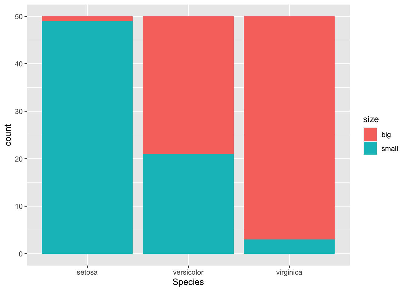
If you prefer to visualize information technology in terms of proportions (so that bars all have a tiptop of 1, or 100%):
ggplot(dat) + aes(x = Species, fill = size) + geom_bar(position = "make full") 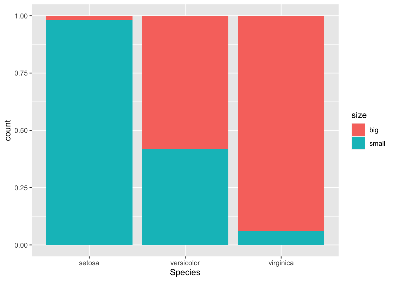
This 2nd barplot is specially useful if there are a different number of observations in each level of the variable drawn on the \(x\)-axis because it allows to compare the two variables on the aforementioned footing.
If you adopt to take the bars next to each other:
ggplot(dat) + aes(x = Species, fill = size) + geom_bar(position = "dodge") 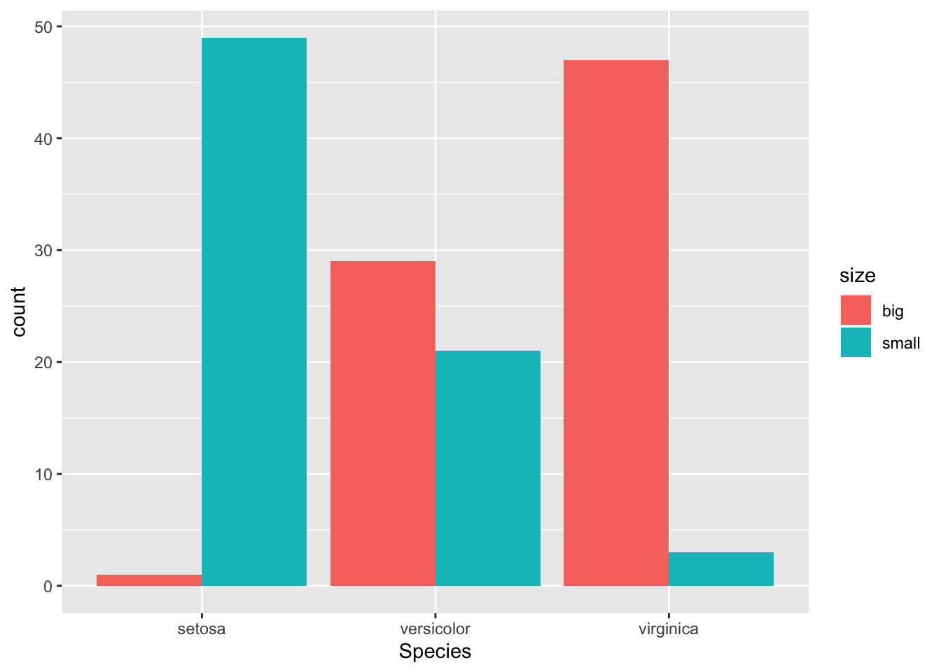
See the article "Graphics in R with ggplot2" to acquire how to create this kind of barplot in {ggplot2}.
Chi-square test of independence in R
For this instance, nosotros are going to examination in R if there is a relationship between the variables Species and size. For this, the chisq.examination() office is used:
examination <- chisq.exam(table(dat$Species, dat$size)) examination ## ## Pearson'southward Chi-squared test ## ## data: table(dat$Species, dat$size) ## X-squared = 86.035, df = ii, p-value < 2.2e-16 Everything you demand appears in this output:
- the title of the test,
- which variables have been used,
- the test statistic,
- the degrees of freedom and
- the \(p\)-value of the test.
You can also retrieve the \(\chi^2\) test statistic and the \(p\)-value with:
examination$statistic # examination statistic ## X-squared ## 86.03451 test$p.value # p-value ## [i] ii.078944e-nineteen If you need to observe the expected frequencies, use test$expected.
If a warning such every bit "Chi-squared approximation may be incorrect" appears, it means that the smallest expected frequencies is lower than 5. To avert this issue, you can either:
- gather some levels (particularly those with a small number of observations) to increase the number of observations in the subgroups, or
- use the Fisher's verbal test
The Fisher's verbal examination does not crave the assumption of a minimum of 5 expected counts in the contingency table. It can be applied in R thanks to the function fisher.test(). This test is like to the Chi-foursquare test in terms of hypothesis and interpretation of the results. Learn more about this examination in this article dedicated to this type of test.
Talking about assumptions, the Chi-square test of independence requires that the observations are independent. This is unremarkably not tested formally, but rather verified based on the design of the experiment and on the good control of experimental conditions. If you are not certain, ask yourself if one observation is related to another (if i observation has an touch on another). If not, it is most likely that you have independent observations.
If y'all take dependent observations (paired samples), the McNemar's or Cochran'south Q tests should be used instead. The McNemar's examination is used when we want to know if there is a significant change in ii paired samples (typically in a written report with a measure before and after on the same subject) when the variables have simply two categories. The Cochran's Q tests is an extension of the McNemar'due south exam when nosotros have more than than two related measures.
For your information, there are three other methods to perform the Chi-square exam of independence in R:
- with the
summary()function - with the
assocstats()office from the{vcd}parcel - with the
ctable()role from the{summarytools}parcel
# 2d method: summary(table(dat$Species, dat$size)) ## Number of cases in table: 150 ## Number of factors: 2 ## Exam for independence of all factors: ## Chisq = 86.03, df = 2, p-value = 2.079e-19 # tertiary method: library(vcd) assocstats(tabular array(dat$Species, dat$size)) ## Ten^2 df P(> X^ii) ## Likelihood Ratio 107.308 2 0 ## Pearson 86.035 2 0 ## ## Phi-Coefficient : NA ## Contingency Coeff.: 0.604 ## Cramer's V : 0.757 library(summarytools) library(dplyr) # fourth method: dat %$% ctable(Species, size, prop = "r", chisq = TRUE, headings = Imitation ) %>% print( method = "return", style = "rmarkdown", footnote = NA ) 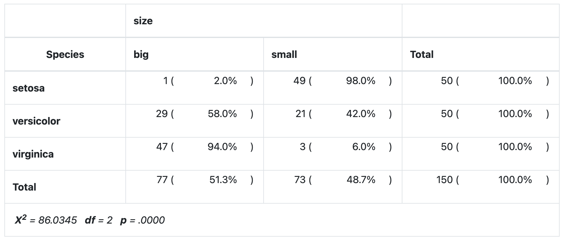
Every bit you lot can meet all four methods requite the aforementioned results.
If y'all do not have the aforementioned p-values with your data beyond the different methods, brand sure to add the correct = Imitation argument in the chisq.test() function to prevent from applying the Yate'southward continuity correction, which is applied by default in this method.1
Conclusion and interpretation
From the output and from test$p.value we see that the \(p\)-value is less than the significance level of 5%. Like whatsoever other statistical test, if the \(p\)-value is less than the significance level, we can decline the zilch hypothesis. If yous are not familiar with \(p\)-values, I invite you to read this section.
\(\Rightarrow\) In our context, rejecting the zilch hypothesis for the Chi-square test of independence means that there is a pregnant relationship betwixt the species and the size. Therefore, knowing the value of one variable helps to predict the value of the other variable.
Combination of plot and statistical test
I recently discovered the mosaic() function from the {vcd} package. This function has the advantage that it combines a mosaic plot (to visualize a contingency table) and the result of the Chi-square test of independence:
library(vcd) mosaic(~ Species + size, direction = c("5", "h"), data = dat, shade = True ) 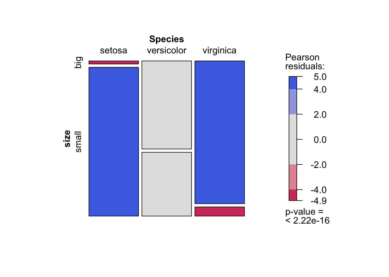
Every bit you can see, the mosaic plot is similar to the barplot presented above, but the p-value of the Chi-foursquare exam is too displayed at the bottom right.
Moreover, this mosaic plot with colored cases shows where the observed frequencies deviates from the expected frequencies if the variables were independent. The red cases means that the observed frequencies are smaller than the expected frequencies, whereas the blue cases means that the observed frequencies are larger than the expected frequencies.
An alternative is the ggbarstats() function from the {ggstatsplot} package:
# load packages library(ggstatsplot) library(ggplot2) # plot ggbarstats( data = dat, x = size, y = Species ) + labs(caption = NULL) # remove explanation 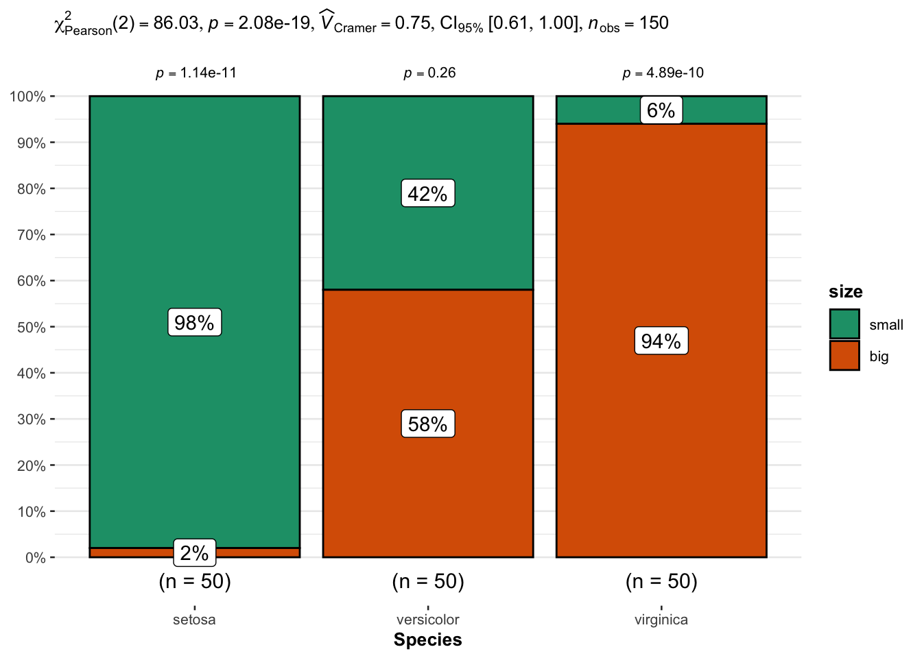
From the plot, information technology seems that big flowers are more likely to belong to the virginica species, while small flowers tend to belong to the setosa species. Species and size are thus expected to exist dependent.
This is confirmed thank you to the statistical results displayed in the subtitle of the plot. There are several results, only we tin can in this case focus on the \(p\)-value which is displayed after p = at the top (in the subtitle of the plot).
Every bit with the previous tests, we reject the null hypothesis and we conclude that species and size are dependent (\(p\)-value < 0.001).
Thanks for reading. I promise the commodity helped you to perform the Chi-square test of independence in R and interpret its results. If you would similar to learn how to do this examination past mitt and how it works, read the article "Chi-square test of independence past manus".
As always, if you have a question or a suggestion related to the topic covered in this commodity, please add it as a comment and so other readers can benefit from the discussion.
Liked this post?
Get updates every time a new article is published.
No spam and unsubscribe someday.
Share on:
Is It Different to Read a Chi Square Table Than a T Test Table
Source: https://statsandr.com/blog/chi-square-test-of-independence-in-r/